Managing Risk in Investment Portfolios - A Guide to Calculating VAR and CVAR
Source Code: GitHub
Discussing importance & implementation on VAR and CVAR using Python
- What is Value-at-risk (VAR)?
- Types of VAR
- What is Conditional Value-at-Risk (CVaR)?
- Calculate VAR and CVAR in Python
- Comparison between Different Methods
- Conclusion
Risk management is crucial in portfolio optimization when talking about investment. Knowing how much risk we can tolerate, we can make informed investment decisions. Value-at-risk (VAR) is one of the most widely used measures of risk and has become a standard measure of risk used by banks and other financial institutions around the world. In fact, VAR (RiskMetrics) was launched within JP Morgan prior to 1994.
In this blog, we will explore the concept of VAR and Conditional Value-at-Risk (CVaR) in detail and demonstrate how they can be used to calculate risk in financial portfolios. Topics involve the basics of VAR, how to calculate it using different methods (historical, parametric, and simulation), and how to interpret the results. After reading this blog, you’ll have a solid understanding of VAR and its implementation and importance in risk management.
What is Value-at-risk (VAR)?
Value at Risk (VAR) is a statistic used to measure and manage the extent of possible financial losses within a firm, portfolio, or a certain period, with a certain level of confidence. Essentially, VAR estimates the worst-case scenario or the potential downside risk of an investment. This metric is commonly computed using historical simulation, parametric modeling, and Monte Carlo simulation.
VAR has its strengths and weaknesses, on one hand, it is simple to use and it allows quick estimates of the risk level in their portfolio. The portfolio manager can use VAR to access the risk and make informed decisions. On the other hand, it assumes the return follows a certain distribution and does not account for extreme events that may occur. In addition, VAR does not provide any information about the potential gains but rather only estimates the expected loss in the worst-case scenario.
Hypothetical VAR Example
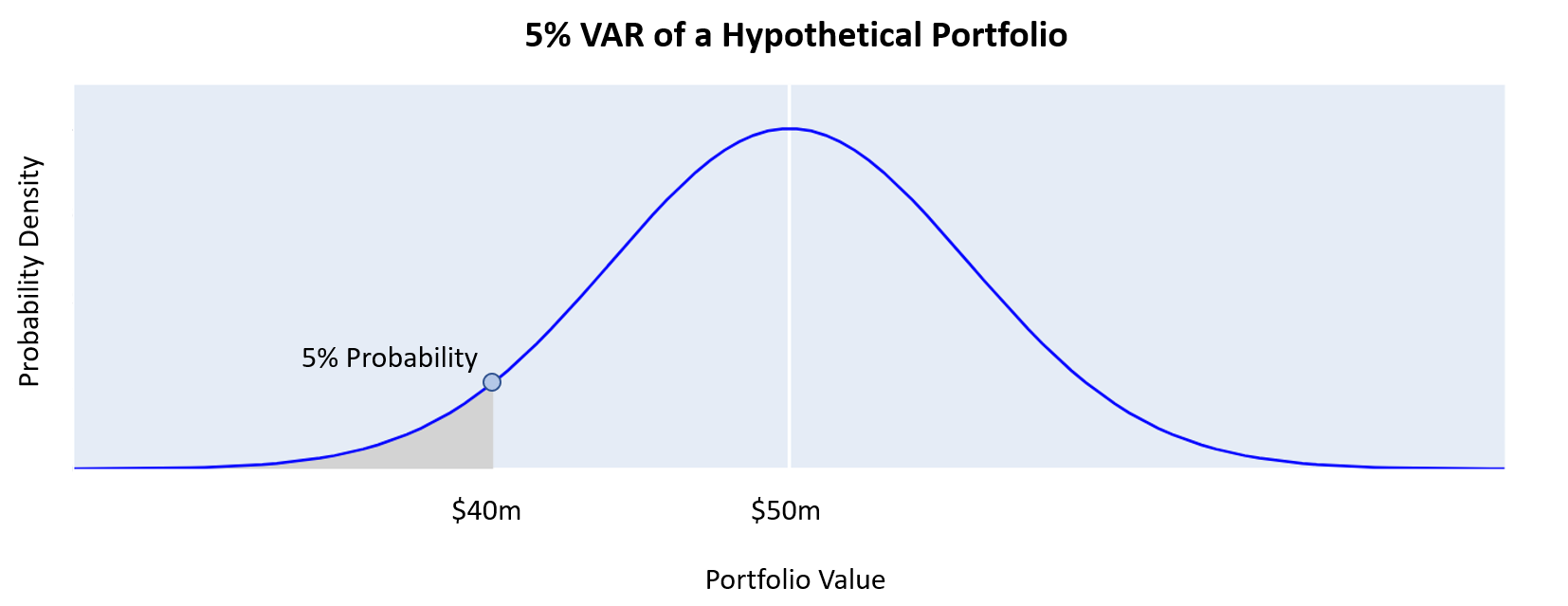
From the hypothetical portfolio shown above, this portfolio is expected to return $50M, there is a 5% chance that the portfolio value will be below $40M. The VAR for this portfolio at the 5% confidence level is $10M ($50M - $40M). This implies that there is a 95% chance that the portfolio will not lose more than $10M over the specified time horizon. This means that the portfolio is expected to perform within a range of $40M to $60M with a 95% confidence level, based on the assumption that the portfolio returns are normally distributed and that past performance is a good indicator of future performance.
Types of VAR
There are three common methods for calculating the VAR given a confidence level and time horizon.
- Historical VAR: it estimates the potential loss based on historical market data and assumes that future market movements are similar to those that have happened in the past. This method is often used by smaller firms with limited data resources. However, it does not take into account extreme market events or sudden changes in market conditions.
- Parametric VAR: it calculates the potential loss with statistical models considering the distribution of market returns. This method is more advanced than historical VAR and can offer a more accurate estimate of the VAR. However, it assumes that market returns follow a specified statistical distribution, which may not always be the case in the real stock market. Moreover, it can be sensitive to anomalies in the data.
- Monte Carlo Simulation: the most accurate approach among these three, it generates a large number of the possible outcome and measures the likelihood of each scenario. Although it is capable of accounting for a wide range of market conditions, it can be resource-intensive and require a large amount of data to generate reliable results.
After discussing the three main kinds of VAR estimations, we will explore each of them in detail and work with sample data in Python. This hands-on approach will allow us to gain a practical understanding of how each method works and when it is most appropriate to use them.
What is Conditional Value-at-Risk (CVaR)?
Before delving deeper into the technical aspects of calculating VAR, it is important to explore a key concept in VAR, which is Conditional Value at Risk (CVAR). Understanding CVAR will enhance our knowledge of measuring risk effectively in combination to better inform risk management decisions.
Conditional Value at Risk (CVAR), aka Expected Shortfall (ES), is a risk measure that provides a complete and advanced view of potential losses than VAR. While VAR only measures the maximum loss given a confidence level, CVAR considers the entire loss proportion exceeding the VAR threshold.
CVAR gave us the expected value of losses beyond the VAR threshold, given that the losses exceed this threshold. We will use the example defined in the previous section, if the VAR for a particular portfolio is $40 million at a 95% confidence level, the CVAR would be the expected loss amount if the portfolio lost more than $40 million at a 95% confidence level, assuming the mean portfolio value is $50 million.
Pros & Cons of CVAR
The main advantage of CVAR is that it provides a more realistic estimate of potential losses, especially when there is more likely to be an extreme loss. Given that CVAR takes into account the full distribution of losses above the VAR threshold, it has the potential to capture risks in the tail that may be overlooked by VAR. However, one disadvantage of using CVAR increases the computation complexity, especially when the portfolio is not normally distributed.
Overall, while VAR is still extensively utilized in risk management, CVAR can offer a more comprehensive and precise evaluation of potential losses in particular scenarios. Therefore, risk managers must be aware of the strengths and weaknesses of both measures and opt for the appropriate one that suits their business needs.
Calculate VAR and CVAR in Python
In this section, we will explore the step-by-step process of using Python to calculate VAR and CVAR for a portfolio consisting of four stock tickers with equal weight for simplicity. We will start by loading the data using the yfinance package and then go through the estimates one by one. By the end of this tutorial, you will have a clear understanding of how to apply VAR calculations to real-world financial risk management scenarios.
Data Collection
First, we import all the necessary Python packages, including data collection, data wrangling, and statistics.
import numpy as np
import pandas as pd
import matplotlib.pyplot as plt
import seaborn as sns
import yfinance as yf
import datetime
from scipy.stats import norm
Second, we will be using the yfinance package to collect stock data. We will be selecting the adjusted close price per day from the time range of 2018-01-01 to 2023-01-01. This will give us the necessary data to perform our calculations and analyze the risk associated with the stock.
# Define start and end date
start_date = datetime.datetime(2018, 1, 1)
end_date = datetime.datetime(2023, 1, 1)
# Download stock data using yfinance, sample stock tickers: [AAPL (Apple), Meta, C (Citi group), DIS (Disney)]
df = yf.download(['AAPL','META', 'C', 'DIS'], start=start_date, end=end_date)['Adj Close']
df.index = pd.to_datetime(df.index)
df.head()
| AAPL | C | DIS | META | |
|---|---|---|---|---|
| Date | ||||
| 2018-01-02 | 40.888062 | 62.809460 | 108.726059 | 181.419998 |
| 2018-01-03 | 40.880947 | 63.003731 | 109.192848 | 184.669998 |
| 2018-01-04 | 41.070835 | 63.780819 | 109.144241 | 184.330002 |
| 2018-01-05 | 41.538441 | 63.696362 | 108.551003 | 186.850006 |
| 2018-01-08 | 41.384151 | 62.953033 | 106.994995 | 188.279999 |
EDA
Before diving into the calculations, let’s take a quick look at our data set. We’ll start by creating a time series plot of the adjusted close price of our selected stock, using data from 2018-01-01 to 2023-01-01. This will give us a visual representation of the stock’s price movements over time, which will be helpful in understanding the calculations we’ll perform later.
ax = df.plot.line(xlabel="Time", ylabel="Adjusted Close Price")
ax.set_title("Adjusted Close Price for Sample Stock Tickers")
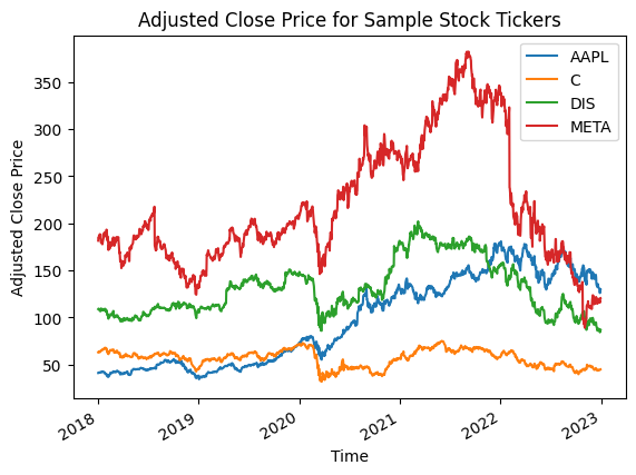
As we can see from the plot, META has the highest adjusted close price, with peaks in 2021, but the price drops significantly starting in 2022. In contrast, Citi Group has the lowest price overall throughout the given time period. It is interesting to note that all four stocks show a sudden drop in the first quarter of 2020, suggesting that the COVID-19 pandemic had a significant impact on the stock market. This quick analysis gives us a sense of the overall trends and movements in our data.
Since we are comparing the relative size of price changes across different assets and time periods, it is necessary to use percentage changes instead of the close price directly. This will allow us to analyze the changes in each asset without mismeasuring the effect due to scale differences. In the experiment below, we will use the percentage change and apply equal weight for simplicity.
Based on the percentage change histogram, most of the changes are within the -0.05 to 0.05 percentage range.
Historical Method
Now that we have a sense of the overall trends, we will calculate the VAR and CVAR using the historical method as a quick start. Recall that the historical method assumes that future returns will follow a similar distribution to historical returns.
Assuming a 1-day time horizon and a confidence level of 95%, let’s calculate the VaR and CVaR for our portfolio.
# Assume initial portfolio value
initial_portfolio = 100000

# Obtain percentage change per stock
returns = df.pct_change()

# Calculate the portfolio returns as the weighted average of the individual asset returns
weights = np.full((4), 0.25) # assuming equal weight
port_returns = (weights * returns).sum(axis=1) # weighted sum

# Calculate the portfolio's VaR at 95% confidence level
confidence_level = 0.95
# Calculate P(Return <= VAR) = alpha
var = port_returns.quantile(q=1-confidence_level)
# Calculate CVAR by computing the average returns below the VAR level
cvar = port_returns[port_returns <= var].mean()

# Multiply the VaR and CVaR by the initial investment value to get the absolute value
var_value = var * initial_portfolio
cvar_value = cvar * initial_portfolio

print(f"Historical VaR at {confidence_level} confidence level: {var_value:.2f} ({var:.2%})")
print(f"Historical CVaR at {confidence_level} confidence level: {cvar_value:.2f} ({cvar:.2%})")
Historical VaR at 0.95 confidence level: -2873.27 (-2.87%)
Historical CVaR at 0.95 confidence level: -4403.11 (-4.40%)
The historical VaR at 0.95 confidence level is calculated to be -2.87% or -2873.27 dollars. This means that if we have a portfolio with an initial value of $100,000, there is a 95% chance that the losses on the portfolio in a given day will not exceed $2,873.27. In this case, the historical data suggests that the portfolio is relatively safe, with a low likelihood of large losses.
Similarly, the historical CVaR at 0.95 confidence level is calculated to be -4.40% or -4403.11 dollars. This means that if the portfolio loses more than the VaR, on average, the expected loss is around $4,403.11. In this case, the historical CVaR is higher than the historical VaR, indicating that if the portfolio experiences losses beyond the VaR, the losses are likely to be substantial.
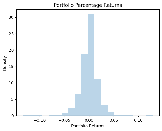
# Plotting
plt.hist(port_returns, bins=20, density=True, alpha=0.3)

# Add VAR CVAR to the histogram
plt.axvline(x=var, color='red', linestyle='--', label=f"VaR: {var:.2%}")
plt.axvline(x=cvar, color='blue', linestyle='--', label=f"CVaR: {cvar:.2%}")

plt.legend()
plt.xlabel("Portfolio Returns")
plt.ylabel("Density")
plt.title(f"Portfolio Percentage Returns")
plt.show()
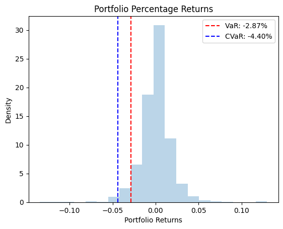
The plot above shows the position of the historical VAR and CVAR in our percentage change distribution, which is in the lower tail of the plot.
Parametric Method (Variance-Covariance)
Since the variance-covariance approach assumes a given distribution (normal distribution in our case) for the portfolio returns, it does not require any time horizon but the mean and standard deviation of the portfolio returns.
# Assume initial portfolio value
initial_portfolio = 100000

# Obtain percentage change per stock
returns = df.pct_change()

# Calculate mean and covariance matrix of returns
mean_returns = returns.mean()
cov_matrix = returns.cov()

# Calculate portfolio mean return and standard deviation
weights = np.full((4), 0.25)
port_mean_return = (weights * mean_returns).sum()
port_std_dev = np.sqrt(weights.T @ cov_matrix @ weights)

# Calculate VaR and CVaR using the parametric method
confidence_level = 0.95
z_score = norm.ppf(q=1-confidence_level)
var = - (norm.ppf(confidence_level)*port_std_dev - port_mean_return)
cvar = 1 * (port_mean_return - port_std_dev * (norm.pdf(z_score)/(1-confidence_level)))

var_initial = initial_portfolio * var
cvar_initial = initial_portfolio * cvar

print(f"Parametric VaR at {confidence_level} confidence level: {var_initial:.2f} ({var:.2%})")
print(f"Parametric CVaR at {confidence_level} confidence level: {cvar_initial:.2f} ({cvar:.2%})")
Parametric VaR at 0.95 confidence level: -2979.65 (-2.98%)
Parametric CVaR at 0.95 confidence level: -3744.60 (-3.74%)
From the result above, we can conclude that if we have a portfolio with an initial value of $100,000, there is a 95% chance that the losses on the portfolio in a given day will not exceed $2,979.65. In this case, the portfolio is also safe, with a low likelihood of large losses, which has a similar risk as using the historical approach (-2.87%).
Similarly, the parametric CVaR at 0.95 confidence level is calculated to be -3.74% or -3744.60 dollars, meaning the average loss beyond the parametric VAR is around $3,744.60. Again, the parametric CVAR is similar to the one in the previous approach.
plt.hist(port_returns, bins=20, density=True, alpha=0.3)

# Add VAR CVAR to the histogram
plt.axvline(x=var, color='red', linestyle='--', label=f"VaR: {var:.2%}")
plt.axvline(x=cvar, color='blue', linestyle='--', label=f"CVaR: {cvar:.2%}")

plt.legend()
plt.xlabel("Portfolio Returns")
plt.ylabel("Density")
plt.title(f"Portfolio Percentage Returns")
plt.show()
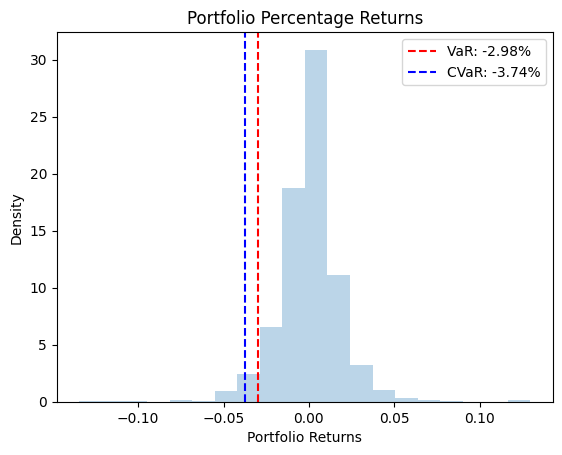
The pattern of the parametric VAR and CVaR is similar to that of the historical values.
Monte Carlo Simulation
The Monte Carlo simulation generates the stock price (random walk) for a predefined number of days (T = 252 trading days in a year) and simulation (n = 400).
Assumes the daily returns follow the multivariate normal distribution, we will use np.normal with covMatrix to simulate the stock’s percentage change
After getting the simulated percentage change, we can find the quantile of these data and calculate the VAR accordingly.
Let’s simulate the percentage change first.
# Set random seed for reproducibility
np.random.seed(123)

initialPortfolio = 100000

n_simulation = 400 # number of simulations
T = 252 # number of trading days in a year
weights = np.full((4), 0.25)
meanM = np.full(shape=(T, len(weights)), fill_value=mean_returns).T

sim_pct_change = np.full(shape=(T, n_simulation), fill_value=0.0)
for m in range(n_simulation):
    # Generate random numbers matrix for each day in the timeframe T and each stock in the portfolio
    Z = np.random.normal(size=(T, len(weights)))
    # Obtain the Cholesky decomposition of the covariance matrix
    # factoring the covariance matrix into the product of a lower triangular matrix (L) and its conjugate transpose (L*)
    L = np.linalg.cholesky(cov_matrix)
    # Calculate daily percentage change using the Cholesky decomposition
    daily_pct_change = meanM + np.inner(L, Z)
    # Calculate the simulated portfolio percentage change for each day in the timeframe T
    sim_pct_change[:,m] = np.inner(weights, daily_pct_change.T)
Let’s visualize the simulated percentage change and its mean, 5th and 95th Percentile.
# Plotting
plt.plot(sim_pct_change)

plt.axhline(np.percentile(sim_pct_change,5), color='r', linestyle='dashed', linewidth=1, label='5th Percentile')
plt.axhline(np.percentile(sim_pct_change,95), color='g', linestyle='dashed', linewidth=1,  label='95th Percentile')
plt.axhline(np.mean(sim_pct_change), color='b', linestyle='solid', linewidth=1, label='Mean')

plt.legend()
plt.ylabel('Portfolio Percentage Change')
plt.xlabel('Days')
plt.title('MC Simulation of a Stock Portfolio Percentage Change')
plt.show()
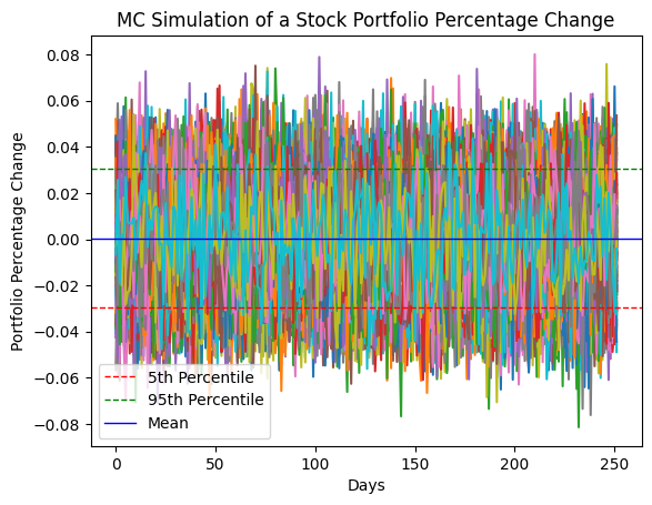
From the above plot, we can observe that the 5th and 95th percentile values are similar to the historical and parametric VAR, around 2% to 3%. It is worth noting that the mean percentage change is close to 0%, indicating that the portfolio is expected to neither gain nor lose on average. This could mean that our chosen stock is diversified enough as we have stocks from different sectors, namely Technology, Communication Services, and Financial Services. In addition, the stocks are also not subject to large fluctuations. One possible reason is that our stocks have lower volatility and risk in the portfolio.
We can now convert the simulated percentage change to actual portfolio returns, considering the initial portfolio amount of $100,000.
confidence_level = 0.95
# Convert sim_returns to dataframe
port_pct_change = pd.Series(sim_pct_change[-1,:])
# Calculate the VAR and CVAR at 95% confidence level of the portfolio percentage change
mcVAR = port_pct_change.quantile(1 - confidence_level)
mcCVAR = port_pct_change[port_pct_change <= mcVAR].mean()

# Create data frame fill with 0
portfolio_returns = np.full(shape=(T, n_simulation), fill_value=0.0)

# Convert the percentage change to actual portfolio value
for m in range(n_simulation):
    portfolio_returns[:,m] = np.cumprod(sim_pct_change[:,m]+1)*initialPortfolio

# Select the last simulated trading day records
last_portfolio_returns = portfolio_returns[-1, :]
# Calculate the VAR and CVAR at 95% confidence level of the portfolio returns
mc_var_returns = np.percentile(last_portfolio_returns, 5)
mc_cvar_returns = last_portfolio_returns[last_portfolio_returns <= mc_var_returns].mean()

print(f"Monte Carlo VAR at 95% confidence level: ${mc_var_returns:.2f} ({mcVAR:.2%})")
print(f"Monte Carlo CVAR at 95% confidence level: ${mc_cvar_returns:.2f} ({mcCVAR:.2%})")
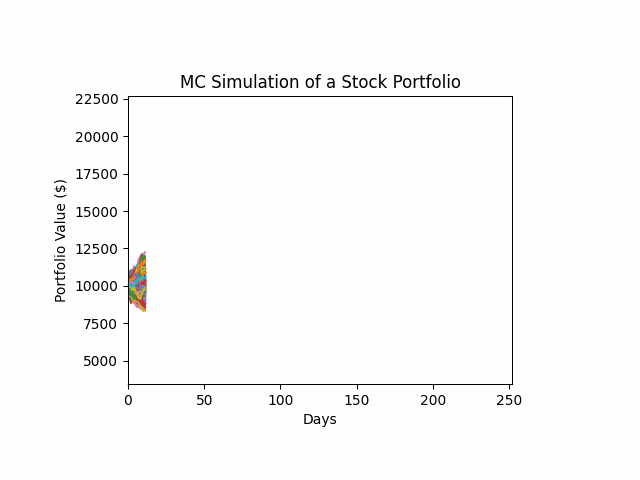
Monte Carlo VAR at 95% confidence level: $64215.77 (-3.09%)
Monte Carlo CVAR at 95% confidence level: $55416.67 (-3.74%)
There is a 95% probability that the portfolio will not lose more than 3.09% ($64215.77) over a given period of time (1 year), based on the Monte Carlo simulation. The Monte Carlo VAR and CVAR show a similar range as the historical and parametric one, with values ranging from -2% to -3%.
# Plotting
plt.plot(portfolio_returns)

plt.axhline(mc_var_returns, color='r', linewidth=1, label=f'VAR: ${mc_var_returns:.2f}')
plt.axhline(mc_cvar_returns, color='g', linewidth=1,  label=f'CVAR: ${mc_cvar_returns:.2f}')

plt.legend(loc='upper left')
plt.ylabel('Portfolio Value ($)')
plt.xlabel('Days')
plt.title('Monte Carlo Simulation of the Stock Portfolio')
plt.show()
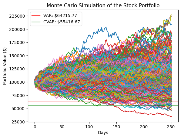
The Monte Carlo simulation generates 400 simulated portfolio values for each of the 252 trading days. The calculated VAR and CVAR values at the 95% confidence level are based on the distribution of these simulated portfolio values. From the plot, we can see that both values are around 5% of the simulated portfolio proportion at the 95th percentile, which is observed on the 252nd day of the simulation. This suggests a reasonable estimate of potential portfolio losses at this confidence level.
Comparison between Different Methods
The historical approach uses past returns data to estimate the VAR. It calculates the n-th percentile, such as the 5th percentile, to determine the VAR for a given confidence level, for example, 95%. This method is straightforward to implement and does not require any distribution assumptions. However, it is limited by the relevance and availability of historical returns, and it assumes that the past is representative of the future.
The parametric VAR approach assumes that returns follow a normal distribution. It estimates the VAR using statistical formulas based on the mean and standard deviation, as well as the covariance matrix of the returns data. This method can be more efficient than the historical approach, but the normal distribution assumption may not always be valid in the real stock market. Additionally, this method is sensitive to outliers in the data.
The Monte Carlo simulation approach calculates the VAR by simulating possible outcomes of the portfolio value. This method can account for complex interactions between assets and does not rely on any distribution assumptions. However, it is computationally intensive, and the results can be sensitive to the model’s assumptions and inputs.
The CVAR is calculated in the same way in all three approaches and measures the expected loss beyond the VAR threshold.
Conclusion
After reading this blog, you should have a clear understanding of how to calculate VAR and CVAR in portfolio management using the three approaches discussed: historical, parametric, and Monte Carlo simulation. The historical approach is simple to implement but requires a sufficient amount of past portfolio returns. The parametric method may be more appropriate for businesses that have limited historical data but it assumes a normal distribution of the stock value. The Monte Carlo simulation is suitable for businesses that require a more comprehensive analysis of potential risks and has high computational resources. Selecting the appropriate VAR calculation method depends on a thorough assessment of the company’s risk profile and requirements, as well as the benefits and drawbacks of each method.
For those who are interested in replicating the analysis, please feel free to visit this Jupyter Notebook
Share on: